Most Dominant Single-Season NHL Scoring Forward?

It’s no open netter. One actuary laces up his statistical skates to find an answer

By BEN MECKLER February 2026

---

Photo credit: Shutterstock

As a corporate actuary for a Canadian life insurer, I focused my attention on topics such as IFRS 17, Financial Condition Testing and ORSA. Now retired, I’ve redirected my energy to explore which NHL forward had the most dominant goal-scoring season. Hockey is our national pastime, notwithstanding the fact that it’s been 32 years (as of 2025) since a Canadian team last hoisted the Stanley Cup. The drought for the Toronto Maple Leafs is a disastrous 58 years. But enough wallowing in self-pity.

To be sure, there may be many ways to address the question of scoring dominance. This article reflects the approach of one actuary, whose motivation is a combined passion for the game and an affinity for numerical analysis.

At first blush, one might point to the 1981–1982 season, when Wayne Gretzky scored an eye-popping 92 goals, a record that has held up for over four decades. Yet, we should not rush to a conclusion, as there are factors that may obfuscate seasonal comparisons. For starters, the number of games in a season has changed. In the 1940s, a season consisted of 50 games, but in more recent years, it has stabilized at 82 games. There were also shortened seasons due to lockouts and pandemics.

Another reason for not relying strictly on absolute raw totals is that dominance needs to be judged based on the degree to which a forward exceeded his peers. If several players rack up decent numbers in the same season, the relative dominance of the top scorer becomes diluted. There are factors that have facilitated more goal production, such as changes to the rules, more sophisticated coaching, better equipment, etc. However, there are factors that may lead to fewer goals, such as the increase in size of defensemen and goalies, as well as changes in goaltending techniques.

The number of teams competing in a season shouldn’t be ignored. It’s more challenging to rise to the top in a field of 32 teams of players than when there were only six.

So, we need an approach that looks at both absolute and comparative factors, affected by season length and number of teams. At this point, I figured that it was time to lace up the figurative statistical skates, with a “goal” of determining who had the most dominant season. At least, I would “take a shot” at it. (I couldn’t resist these puns.)

Scope and data source

As with many an actuarial challenge, I first needed to define the scope. I decided to limit the review to the period beginning with the 1942–1943 season (the start of the Original Six era and when seasons had 50 games¹) and ending with the 2024–2025 season.

My next executive decision was to restrict the focus to goal production. While assists are important, they are not going to be included in this analysis.

The other issue to be resolved is the source for the data. I used hockey-reference.com. It has the relevant information for players by season, which can be exported into Excel for analysis. I did a number of spot checks against the data at NHL.com, just to satisfy myself about the data integrity.

Initial screening

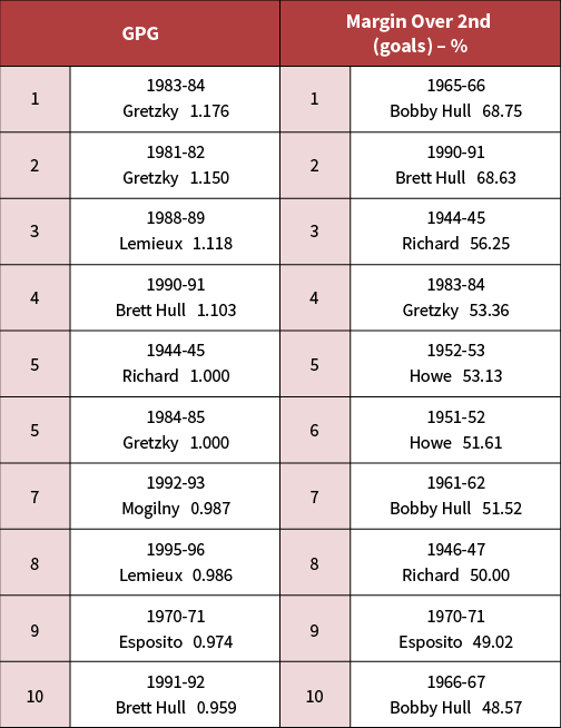
Rather than doing a deep dive of all years, I decided to do an initial screening based on only a limited and readily accessible data for each season: the top scorer’s goals, number of games played and the second-highest goals. If there was a tie for the top scorer, I used the one who had a higher Goals per Game (GPG). I then established the following two initial metrics, meant to capture a blend of dominance across and within seasons:

• Top scorer’s GPG
• Margin over second in goals, expressed as a percentage

These results were then sorted by each metric. Table 1 shows the top 10 for each metric:

Table 1: Initial metrics

To proceed to the next round for further analysis, I established screening criteria. To be eligible, the player/season would need to satisfy a minimum of one of the following:

• Place in the top four in at least one category
• Place in the top ten in both categories

Table 2 shows the qualifiers, in chronological order:

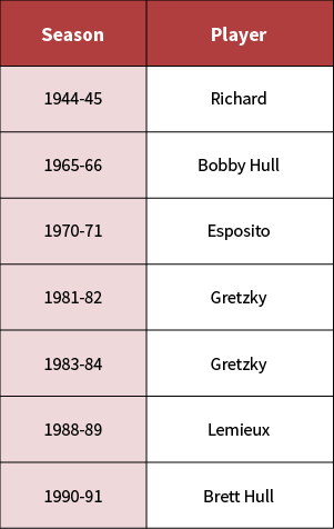
For the most part, this “Magnificent Seven” provided an interesting cross-section of different eras. Included in this list were: Maurice “Rocket” Richard’s iconic 1944–1945 season (50 goals in 50 games); Bobby “The Golden Jet” Hull’s 1965–1966 season, where his margin percentage over the second tops the list; Phil Esposito’s 1970–1971 season (his six-season streak as the top goal scorer is unmatched); two seasons of Wayne Gretzky in his early 1980s prime; followed by Mario Lemieux (1988–1989) and Brett Hull (1990–1991), both in peak form.

Notice that no 21st century player made the initial cut. To address this potential deficiency, I added two more to the list: Austin Matthews’ 2023–2024 season, where he scored 69 goals (tops this century); and Alex Ovechkin’s 2007–2008 season (his personal best). Also, my initial list only included the players who topped their season in goal production. For the most part, this would correlate closely with the leader that season in GPG. But I recall one glaring exception. In the 1992–1993 season, Lemieux missed approximately a quarter of the games as he was receiving treatment for Hodgkin’s lymphoma². Although he wasn’t first in goals (he was first in points), his 69 goals in 60 games for a GPG of 1.15 was tops that season and tied for second for all seasons³.

The final list for further filtering is shown in Table 3:

Unfortunately, a few legendary players didn’t make the cut, which likely never happened during their careers. These include Gordie Howe, Guy Lafleur (one of my personal favorites), and Sidney Crosby. Their fans shouldn’t feel snubbed. This was meant to be a rarefied list.

Seasonal filtering

With the seasons selected, I filtered the data from hockey-reference.com. First, I restricted the comparative analysis to forwards—defensemen were excluded for consistency. Second, only forwards who played at least half the season were considered. Third, to be eligible for the pool, forwards needed to score a minimum number of goals based on the season’s length. To screen out non-scorers (e.g., enforcers, fourth liners), I applied a minimum goal threshold: 0.075 x season games, rounded.

Lastly, as with typical actuarial assignments, data cleansing was necessary. The most significant issue here was to avoid double-counting if a forward played for multiple teams in a season.

New metrics

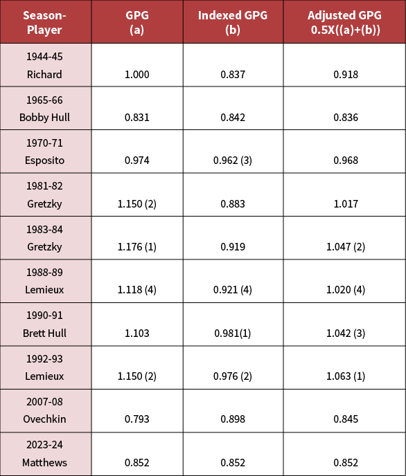
With the filtered data loaded in Excel, I focused on GPG. Due to the different season lengths, GPG provides a better comparability than raw goals. Even within seasons, GPG addresses anomalies, as noted with Lemieux in 1992–1993. However, some recognition of era differences should be made. A straightforward approach is to incorporate the Average Team Goals Per Game (ATGPG) for each season under review, available at hockey-reference.com.

Setting 2023–2024 as the base season, I computed an index value for any season as the ratio of the base ATGPG to that season’s ATGPG. The resulting indexed GPG would then be the product of the GPG and the index value. To provide a reasonable balance, I used the average of GPG and the indexed GPG to arrive at the Adjusted GPG. The results are shown in Table 4. This approach provided slight boosts to Brett Hull and 1992–1993 Lemieux, whereas Gretzky’s seasons lost some ground.

Table 4: Adjusted GPG (top 4 in parentheses)

For within-season dominance, in the first round, I only compared the leader against the runner-up. For this round, I also included benchmarking the top player’s performance against elite, moderately successful, and average forwards.

For the comparison against the average, I initially considered using Z-scores to measure how far the top scorer was above the mean. However, this measure would only be valid if the distribution is normal or, at least, close to normal. This issue led me to a brief but enjoyable diversion.

Are goals per game normally distributed?

My first step was to calculate the 10 Z-scores and review them for the plausibility of normality. The results are shown in Table 5.

As can be seen, the scores were staggering, with five out of the 10 having a score of at least five. In a truly normal distribution, the probability of drawing a value five standard deviations above the mean is approximately one in 3.5 million, and this happened five times! (In the most extreme of the seasons, the probability is one in 131 million.)

Table 5: Test for normality – GPG

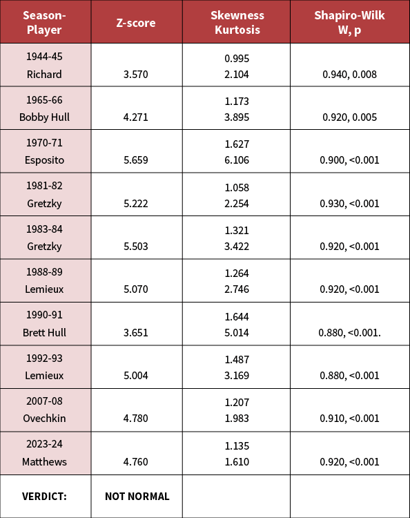
Those results are strongly suggestive that we are not dealing with a normal distribution. But to be thorough, I ran additional tests.

Excel has built-in functions that calculate skewness and kurtosis (excess), the results of which are also displayed in Table 5. As there does not appear to be universal agreement on how to interpret these results⁴, I referred to conservative guidance that, for an assumption of normality or near normality, skewness should be in the range of -1.0 to +1.0⁵ and kurtosis in the range of -2.0 to +2.0⁶. As the results show, none of the seasons passed the test, although a couple came close to the outer bounds.

Feeling like Chuck Norris about to deliver a final punishing roundhouse kick to an already vanquished opponent, I fed the data into the online calculator found at statskingdom.com to perform the Shapiro-Wilk test for normality. In a nutshell, based on the league sizes, the W statistic should be close to 1, with the p statistic above .05⁷. The results, also displayed in Table 5, show that none of the seasons have a p statistic anywhere near the minimum threshold.

The conclusion of this work: we reject the assumption of normality.

I then tested to see if the lognormal distribution was plausible. Given its fatter tail than normal distributions, I figured that lognormal had a decent shot. The results are shown in Table 6:

Table 6: Test for normality – log GPG

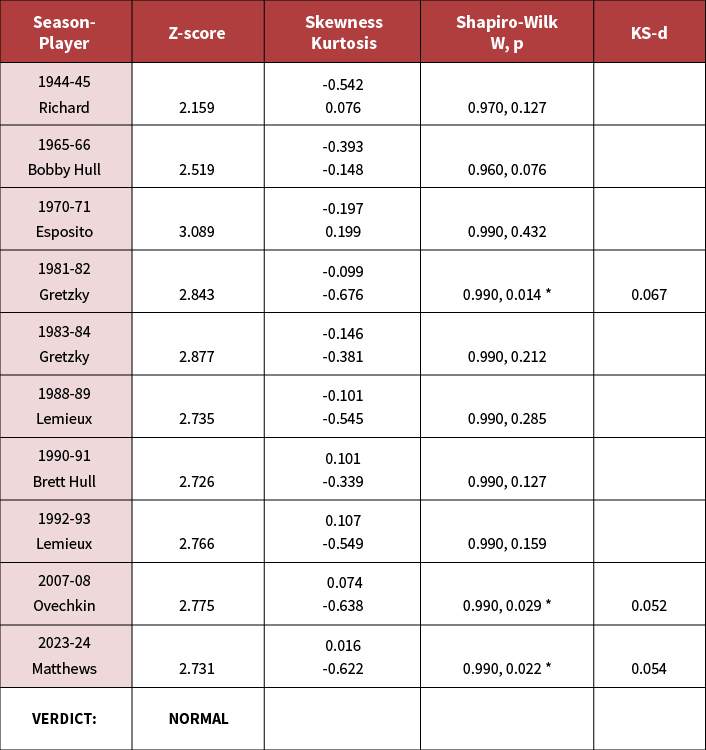
As with Table 5, we started with the Z-scores. This time, however, the results were far more encouraging, with nine out of 10 having Z-scores below 3.0. The lone exception still had a Z-score lower than the smallest Z-score in Table 5.

The next hurdles were the skewness and kurtosis. As can be seen, all tests passed.

We ran into a bit of turbulence, though, with the Shapiro-Wilk test. Although 7 passed, the other 3 (noted with an *) had p-values which were slightly offside. To get a better feel of the degree of dispersion, the online calculator also provided the Kolmogorov-Smirnov statistic, KS-d. The values for the outliers are shown in Table 6. According to the interpretation in the online calculator, the magnitude of the difference between the sample distribution and normal distribution for these cases ranges from “very small” to “small.”

Based on these findings, I concluded that the Z-score of the log of GPG was a suitable metric.

Other metrics

Ranking by the Z-scores of the log of GPG is a useful metric. However, similar to measuring interest rate sensitivities, where we examine key rate durations, for this work, I computed additional measures of peer dominance, i.e., how the leaders performed against “moderate” scorers, “elite” scorers, and the runner-up. For “moderate,” I used the average of the top 50% by GPG, i.e., CTE50. I defined “elite” as the average of the top 10%. To avoid undue influence from the top scorer when the league size was small, I excluded the leader and referred to this adjusted average as CTE90x. I referred to the season’s runner-up simply as 2nd. The excess of the leader over these values was expressed as percentage margins.

Results of the five metrics

The results of the metrics are displayed in Table 7, with the top 4 in each category shown in parentheses:

Table 7: Results

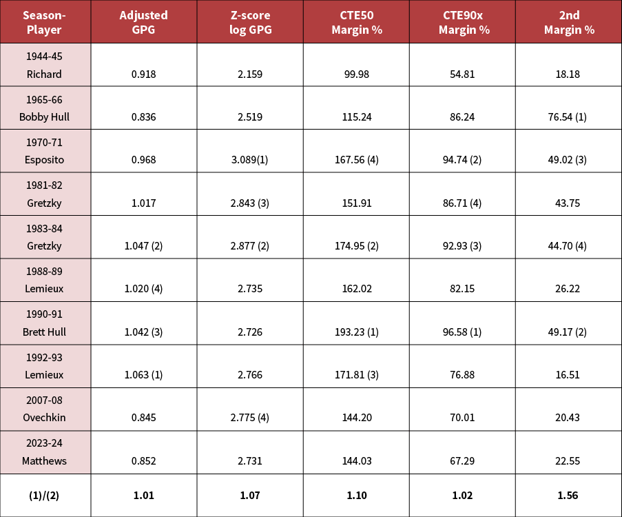
My first inclination was to award 5, 3, 2, and 1 for the top four spots, respectively, which would provide a 2-point margin for the top position. However, upon looking at the ratio of the top to second in one of the metrics, the lead was substantial at 156%. I felt that a 2-point margin wasn’t sufficient to capture the dominance. Accordingly, in this case, the leader received seven points for a 4-point margin.

I should note that with the focus now on GPG, Richard’s relatively strong showing in Table 1 for margin over 2nd was downgraded in Table 7, due to shifting in ordering.

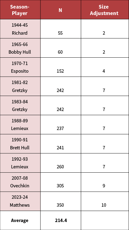
Sixth metric: Size matters

As noted earlier, the league has expanded from 6 to 32 teams. This final metric recognizes that a goal scorer who reaches the apex in goals should be rewarded proportionately to the amount of the competition. Because of its importance, I assigned a top score of 10 points, or double the value of one of the other metrics. The formula I used to achieve this was 6 x N/ (average N), rounded, where N is the eligible player pool for the season and average N is the average of all seasons.

Table 8 shows the scoring for this important metric:

Table 8: Size adjustment

Putting it all together

The scores are tallied and displayed in Table 9:

Table 9: Final scores – and the winner is …

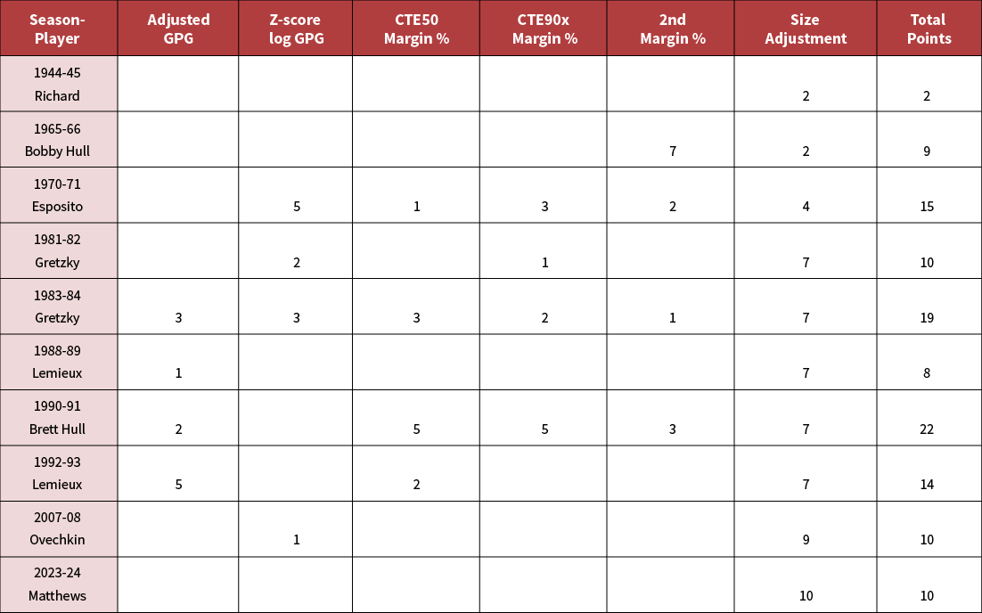
The winner is Brett Hull’s 1990–1991 season with 22 points. Although his Z-score did not make the top 4, his dominance against the upper echelon in his season (tops in two and second in the third) is unmatched, which, together with his third-place finish in Adjusted GPG, vaulted him to the top overall. A close second is Wayne Gretzky’s 1983–1984 season. He is the only one to have been awarded points in every metric. Following him in third place is Phil Esposito’s 1970–1971 season, with points in five metrics. In fourth spot is the 1992–1993 season of Mario Lemieux. Gretzky’s record-breaking 1981–1982 season ranks only in the middle of the pack. His relative dominance was diluted by the strong scoring of others that season. Bobby Hull’s towering performance in 1965–1966 over his immediate rival should have catapulted him to a higher ranking, but he was simply “a big fish in a small (frozen?) pond.”

Final thoughts

This was meant to be a fun exercise. But after a four-decade career, it was ingrained in me to apply some degree of discipline as if it were a work assignment. Many of the critical steps were there: defining the scope, identifying and challenging the data, developing meaningful metrics, doing the calculations, and interpreting the results. The lesson learned, I believe, is that the skill set actuaries bring to the table is not restricted to traditional actuarial roles.

Lastly, it should be stressed that this article strictly considered dominance from the narrowly defined perspective of single-season goal scoring by a forward. There are, of course, other attributes of dominance that can be explored. Examples include consistency at the top, inclusion of assists, plus/minus record, and even the significance/nature of goals scored (e.g., unassisted, short-handed, game winners). Although out of scope for this article, they, too, are worthwhile investigations.

Statements of fact and opinions expressed herein are those of the individual authors and are not necessarily those of the Society of Actuaries or the respective authors’ employers.

Copyright © 2026 by the Society of Actuaries, Chicago, Illinois.