
Practical Use of Bayesian Statistics
Insights for SOA candidates and newcomers to the actuarial profession
July 2023As a now-retired actuary, I love statistics. Moreover, virtually all mathematical analysis, another area I love, can be incorporated one way or another into statistical analysis.
The statistics I learned—covered in the Society of Actuaries (SOA) Probability Exam and often called “frequentist statistics”—showed that by assuming distributions for observations, which are usually described by their parameters, you could estimate a maximum likelihood estimate (MLE) or “best” single value for each of their parameters (say, the mean and standard deviation) and test the validity of a hypothesis.
I recently reintroduced myself to Bayesian analysis, developed centuries ago by Thomas Bayes and “rediscovered” by Pierre Simon Laplace. In addition, I have been so taken by the newer approaches that incorporate powerful computer algorithms, such as Markov Chain Monte Carlo (MCMC), that I have decided to reveal myself as a confirmed Bayesian.
Bayesian Statistics Overview
What makes Bayesian statistics distinct is that you use prior distributions of the parameters (not the data distribution). Again, for the sake of example, let’s say you use the mean and standard deviation as the parameters. Then, you use the data to update the distributions of the parameters.
While predictive modeling is of interest, Bayesian-driven probabilities of future events are also valuable for an actuary because you can use them to develop insurance premiums. Under Bayes, as we get more data, we can update the entire initial probability distribution (the prior distribution) of the parameters (i.e., the mean and standard deviation in this example) and continually update each subsequent posterior distribution of the parameters that results by using this posterior distribution as the prior distribution in the next update. So, under Bayes, we don’t predict an event, but we can get the information we need (i.e., the parameters) to then use to update the distribution of the chance that the event occurs.
Moreover, the focus of Bayesian analysis is different. Again, while much of the newer data analysis such as artificial intelligence (AI) has a prediction focus, Bayesian analysis tries to attack a different problem: credibility.
In the past, I found Bayesian analysis interesting, but as a sideshow. It provided an alternative way to look at a data problem. Still, the path to a solution needed to be simpler for any practical analysis and often involved multiple integrations when there was more than one parameter. I lost interest in trying to use it.
That has changed. This article aims to take us through a quick survey of what Bayesian analysis is and where it can be helpful. But I skip over many steps, assume familiarity with how statistical equations are written and proceed to an example that an actuary with a basic statistical background will find interesting. (In the bibliography at the end of the article, I provide the references I used to learn the basics.)
There is a lot more, like Bayesian hierarchical modeling, ANOVA testing and linear regression, but I cannot cover it all in one article. My goal is to generate interest within our community more than to teach. I am still a novice, and there are plenty of academic articles, books and other resources much better suited to teaching than I am.
So, let’s start with a review of the Bayesian formula for events predicting it will rain, R+, and predicting it will not rain R–. (Hopefully, you will remember this from the Probability Exam, but a review of the syllabus should bring it back.)
To use the rain event as an example, suppose the meteorologist is predicting whether it will rain, R+ or R– .
We let the event they predict rain be R+ and the event R– be the event they predict no rain, where the parameter, say Z+, is “it rains” and Z– is “it doesn’t rain.” We can think of a four-box grid with events listed as rows and parameter results as columns.1
We know from basic logic and basic statistics that P(Z+∩R+) = P(R+∩Z+)
We also know that P(R+∩Z+) = P(R+|Z+) x P(Z+)
So, we can write P(Z+|R+) x P(R+) = P(R+|Z+) x P(Z+)
Rearranging, we get: P(Z+|R+) = (P(R+|Z+) x P(Z+)) / P(R+)
But the practical use for our purposes is to update our beliefs in the parameters of a distribution, and this means we must expand our focus from event R+ to many events (i.e., the new data, D) that can change our beliefs about the one or more Z parameters. The grid then becomes the new data with rows and parameter values of our desired distribution as columns. (This should become clearer in the example.)
We start with the same equation, but we look for the distribution of the parameter(s), Z, or, for example, in the discreet probability case:
P(Z+, D) = P(Z+|D) x P(D)
In our example, D is just the one event R+. But, from the Bayes rule:
P(Z+, D) = P(D, Z+)
P(Z+|D) x P(D) = P(D |Z+) x P(Z+)
In practice, the full data set, D, will arise from all possible values of Z (Z+ and Z – in our example). In other words, we can quickly get P(Z, D), but we need P(D). To get that, we must sum the probabilities of the data over all possible values of Z, P(D) =∑i P(D|Zi ). So, restating the formula in our example:
P(Z +|R+) = (P(R+|Z+) x P(Z+)) / (P(R+) = P(R+|Z+) + P(R+|Z–))
There is an equivalent generalization when continuous distributions are used:
p(Z|D) = p(D|Z) x p(Z) / (∫ p(D|Z) d(Z))
We will see that the denominator can be impossible to calculate directly, especially when the parameters are multidimensional like those found in linear regression. However, no matter how impossible it may be to calculate the denominator directly, it will be just a factor that normalizes the numerator to generate the posterior probability distribution.
Just Another Gibbs Sampler (JAGS) Model Sampling
Traditional Bayesian analysis has long provided solutions to a limited set of problems, but until the advent of the first computer, it could never be applied to more generalized problems. We can see the issue in the generalized continuous case. The only way to solve this problem directly had been to solve for the parameters, z, of the posterior probability distribution directly, and that meant the Bayes formula could only work with distributions that required solving for the precise probability values, p(x).
To find the parameters z (say, mean and standard deviation), the basic Bayesian equation would be:
p(m,sd|D) = p(D|m,sd)*p(m)*p(sd) / p(D)
where p(D) = ∫∫p(D,m,sd) d(m) d(sd)
Even though the integration provides a factor that normalizes the numerator so the posterior distribution would sum to 1, you often face multiple integrals to get the number you need. Moreover, in many areas of data analysis (say, linear regression), you are dealing with a multidimensional probability “hyperplane,” so the number of parameters you need to integrate out of the denominator can easily be 5, 10 or even more, or ∫∫∫∫∫.
This was the state of affairs until the advent of computers and the Manhattan Project. Then, as Monte Carlo analysis developed and the Markov process was added, there was a realization that you could get the parameters you needed by sampling from a posterior density distribution that was the same shape as the probability distribution.
We will need a computer and the MCMC technique for our example.
A Markov process is often called a “random walk,” but the defining characteristic of a Markov chain is that no matter how the process arrives at its present state, the possible future states converge to a fixed state. A Markov chain is developed as a series of events where the probability of something happening depends only on what happened right before it. Monte Carlo is a computational technique based on constructing a random process for a problem and sampling from a sequence of numbers with a prescribed probability distribution.
The central idea is to design a Markov chain model to get the parameters from the prescribed stationary probability density (i.e., the posterior density that is the same shape as the one we need). In the limit, the samples the MCMC method generates will be samples from the desired (target) density (e.g., the posterior distribution).2 The posterior density will usually differ by a scaling factor.3
This stationary distribution is approximated by the empirical samples using the MCMC sampler, and if this stationary state exists, it is unique (by the “ergodic theorem”). That is, there is only one density that is this stationary density (again, this density will give the same parameters as the probability distribution).
I believe there needs to be more background to understand MCMC, but this article focuses on providing an example that shows how MCMC might work in practice. Moreover, we will work with a Gibbs sampler. When you picture this probability problem as a graph, you can imagine a hyperplane with the parameters used for each dimension.
The Gibbs sampler cuts the probability hyperplane into successive two-dimensional, single-parameter planes with the x axis being the current parameter, the other parameter values coming from previous iterations (after starting with initial guesses for them), and the y axis being the probability density. This usually makes the Gibbs sampler much more efficient than other samplers (e.g., Metropolis-Hastings).
So, in the simple case of one normal distribution, we guess at the standard deviation and look for the mean. Then we use that mean and examine a new value for the standard deviation, then use this for a new mean value and so on. We keep doing this until we come to a unique, stable state.
The first Gibbs sampler was Bayesian inference Under Gibbs Sampling (BUGS) and programmed in the R language. Then WinBUGS introduced several improvements, but the code was proprietary, and that led to JAGS (referred to in R as rjags), an open-source code with many of the same bells and whistles.
A Practical Actuarial Case
Next, let us look at a very simple example.4,5,6 A common problem many health and casualty actuaries face is the “credibility problem.” Usually, a company’s standard rates are based on a large database covering a wide range of claim costs. However, an issue often arises where the claim cost experience of a subgroup (either the experience data over the past number of years or the current experience data of a particular subgroup with a special attribute, like occupation) should be used in part or total in setting the new price.
Here is an example: A group of 10 providers all in a given region have had loss ratios significantly less than the standard case. The company’s overall loss ratios are normally distributed, with a mean loss ratio of 80% and a standard deviation of 10%. The loss ratios for the subgroup of 10 providers are also normally distributed, with a mean of 53% with a standard deviation of 27%. You have been asked to determine the credibility and set the loss ratio to be used in the pricing for the group.
First, Z, the data, the actual percentage loss ratios for the group of 10, are:
Z = 76.49%, 34.75%, 60.99%, 75.73%, 8.17%, 51.66%, 70.82%, 42.27%, 89.27%, 16.63%
Z will be set as a vector in JAGS.
Bayesian JAGS Model for Our Example
This Bayesian model assumes the data are normal, with a normal prior for the mean and a uniform prior for the standard deviation. (The ~ is read as “distributed as”.)
Zi ~ N (mean,std2) for i = 1,…,10
{Note: JAGS uses “precision,” the inverse of variance, so in JAGS, we code Z ~ N(mean,std-2)}
Where the priors for mean and std are:
mean ~ Normal (80,102) {Again, in JAGS we use 10-2}
std ~ Unif(0,200) {Unif is the uniform distribution —
(what you use when you don’t have a clue)}
The MCMC method (I’ve left out all the steps in this example to keep things simple) gives us the parameters (mean and standard deviation) from the probability density to use in the standard normal probability distribution. The results are summarized in Figure 1.
Figure 1: Comparison of Mean and Standard Deviations
| Category | Mean | Standard Deviation |
| Company loss ratio (the Prior in Figure 2 below) | 80.00% | 10.00% |
| Group of 10 loss ratio (the SubGroup in Figure 2 below) | 52.68% | 26.98% |
| Bayesian posterior loss ratio (The BayesResult in Figure 2 below) | 66.98% | 34.85% |
We can see the results in the plot in Figure 2.
Figure 2: The BayesResult
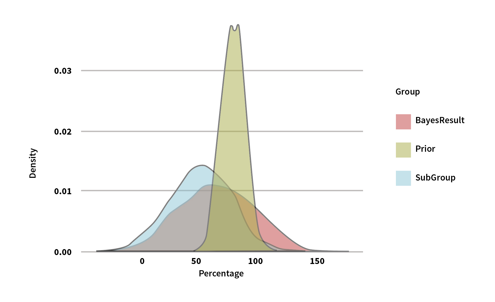
We can see that the Bayesian process assigns 66.98% as a credible loss ratio (i.e., p(mean, std|Z)) for the group. The degree to which the prior and the data MLE influence one another depends on the shape of those two distributions: the skinnier the shape, the more influence it has. So, for example, if the prior were distributed as N(80,202), the Bayesian posterior loss ratio would be 58.22% because the prior is fatter and the data set will have more pull.
To answer the specific question, the loss ratio to use is 66.98% with a 68% confidence range of +-1 x the standard deviation (sd) or +-34.85 from the mean, +-1.645 x sd for 90%, and +- 3 x sd for 99.7%. The reason for the wide range is that we only have 10 data points.
Conclusion
This is a short article with a simple example, and it is merely intended to show the power of Bayesian analysis and the advantage of random sampling. This is not designed to be rigorous, but hopefully useful to an actuary who doesn’t have the time or the background to read the academic-level books and papers to see how it works. Even though the data used here for example’s sake are contrived and the model is very simplified, there are many potential uses in the actuarial field.
There are many distributions that can be modeled in R and JAGS (the Bernoulli, Beta, Gamma and Poisson immediately come to mind). While it is far beyond the scope of what I cover here, the Bayesian analysis can be layered (hierarchal analysis). Then the company-level data subsets can be used to inform the analysis better. Alternatively, the company-level data can become a subset of some higher-level data, such as industry-level data.
But the biggest reason I am trying to develop more interest in Bayesian analysis in our profession is that it plays so well to the key skills that the actuary brings: risk analysis (more than just prediction) and judgment (who better to set the prior?).
Bibliography
Anaconda provides free software for Bayesian analysis and a library of useful programs.
Ghosh, Pulak. Applied Bayesian for Analytics IIMBx. edX.com.
Johnson, Alicia. Bayesian Modeling with JAGS. DataCamp.
Kataria, Sanjeev. Markov Chain Monte Carlo.
Kruschke, John K. 2013. A Tutorial With R, JAGS. In Doing Bayesian Data Analysis, 2nd ed. Academic Press: Elsevier.
Statements of fact and opinions expressed herein are those of the individual authors and are not necessarily those of the Society of Actuaries or the respective authors’ employers.
References:
- 1. Kruschke, John K. 2013. A Tutorial With R, JAGS. In Doing Bayesian Data Analysis, 2nd ed. Academic Press: Elsevier. ↩
- 2. Kataria, Sanjeev. Markov Chain Monte Carlo. ↩
- 3. Ibid. ↩
- 4. Society of Actuaries. Universities & Colleges with Actuarial Programs (UCAP). ↩
- 5. Allen Downey’s blog notes that Nate Silver, founder of fivethirtyeight.com, uses a model similar to the one used in the example in this article in his analysis. (Don’t be discouraged by trying to understand the Python code Downey uses underneath his analysis. It is indecipherable to anyone who is not an expert in Python). Silver’s model is set up differently and will likely have a higher level of sophistication. Still, the normal model works well in the end, as all of Silver’s data comes from polls that assume a normal distribution. ↩
- 6. Johnson, Alicia. Bayesian Modeling with JAGS. DataCamp. (I patterned my example after an example she used.) ↩
Copyright © 2023 by the Society of Actuaries, Chicago, Illinois.